← Back to Blog

Regression Splines for Real Estate Valuation

  • Engineering & Design
Published by Igor Omarov - 23 June 2022
Design & Engineering Regression Splines

At PriceHubble, we work at providing the best tool on the market for real estate property valuation. To do so, we develop what is usually referred to as Automated Valuation Models (AVM). The purpose of an AVM is, given a set of property characteristics, such as the location, the living area, or the floor number, to return the most accurate price estimate for this property.

In this article, we explain how Regression Splines can be useful to effectively build such systems.

Ground Truth

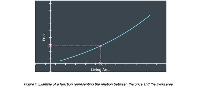
For the sake of simplicity, we consider the problem of estimating the price of a property given its living area. In that case, the AVM can be mathematically represented by a function; i.e. a mapping matching every possible value of the living area to a unique price estimate (figure 1).

Capture d’écran 2022-06-23 à 21.55.41

In practice, all we have is a finite collection of property samples with their living areas and prices which we call the dataset (figure 2). Therefore, the problem of building an AVM amounts to finding the best function representing the relationship between the price and the living area using only this dataset.

Capture d’écran 2022-06-23 à 21.58.16

A naive way to create the AVM would be to use a lookup table built from the dataset. This approach has many limitations, the most important ones being:

  • Extrapolation: The AVM cannot support new living area values not present in the dataset.
  • Definition: Real world data contain properties with different prices for the same living area. In that case, our AVM is ill-defined since the price for a specific living area is not always unique.


In order to build a well defined AVM and avoid the above limitations, we assume the existence of a Ground Truth function. Theoretically, if we have a dataset with an infinite amount of samples covering every possible value of the living area, this function can be defined by mapping each value of the living area to the average price of all samples having this value (figure 3).

Capture d’écran 2022-06-23 à 21.59.41

In the field of statistics, this function is called the regression function. It is the best predictor of the price given the living area. More importantly, it minimizes the mean squared error, which is equal to the average of all errors squared as shown in figure 4.

Capture d’écran 2022-06-23 à 22.01.09

In practice, the ground truth is unknown, but we can still approximate it by finding the function which minimizes the mean squared error over the dataset.


Linear and Polynomial approximations

Finding the function that minimizes the mean squared error among all possible functions is an intractable problem. Therefore, we restrict the search to functions that can be fully defined using a finite number of parameters. This simplifies the problem to finding the set of parameters that minimizes the mean squared error.


Linear approximation

A linear function is fully defined using two parameters: the slope and the intercept (figure 5).

Capture d’écran 2022-06-23 à 22.05.33

The linear approximation (figure 6) is too simple to be able capture the variations of the ground truth. We say that it is underfitting.

Capture d’écran 2022-06-23 à 22.07.14

Polynomial approximation

A more complex class of functions are polynomials. They are defined as the weighted sum of powers (monomials).

Capture d’écran 2022-06-23 à 22.08.16

The highest power is called the polynomial degree. When the degree is fixed, a polynomial is fully defined by a finite number (equals to degree + 1) of weights. In this case, we can create a polynomial approximation by finding the set of weights which minimizes the mean squared error (figure 8).

Capture d’écran 2022-06-23 à 22.10.28

The polynomial approximation is wiggly and tends to rather fit the dataset samples than the ground truth. We say it is overfitting.

Regression Splines approximation

Although polynomials suffer from overfitting, they are still very good local approximators. To take advantage of this property, we can approximate the ground truth using a piecewise polynomial. Namely, we divide the range of our samples into small intervals and approximate the ground truth on each one separately by a different polynomial (figure 9).

Capture d’écran 2022-06-23 à 22.11.41

This approximation is slightly better than the polynomial one, but the function has some points of discontinuity.

Regression Splines

Regression Splines are none other than piecewise polynomials smoothed out in the discontinuity points. Beside being better approximators, this class of functions has many advantages:

  • They can be fully defined with a finite number of parameters
  • Their smoothness can be effectively controlled
  • They can incorporate prior knowledge like monotonicity

B-spline basis

As for polynomials, regression splines can also be written as the weighted sum of a finite number of predefined functions called the B-spline basis functions (figure 10).

Capture d’écran 2022-06-23 à 22.13.16

The spline approximation is created by finding the weights that minimize the mean squared error. The solution is better than the polynomial approximation but still presents some wiggliness.

Capture d’écran 2022-06-23 à 22.14.14


Smoothing

This wiggliness can be reduced by keeping the weights corresponding to neighboring B-spline basis functions close to each other (figure 12).

Capture d’écran 2022-06-23 à 22.15.27

If the weight differences are constrained to stay small, we obtain a smooth approximation (figure 13).

Capture d’écran 2022-06-23 à 22.17.41


Monotonic constraints

In some cases, we have prior knowledge which is not necessarily reflected in the data. In this simple example, the price should always increase when the living area increases. This is not perfectly the case in our approximation (there is a plateau toward the middle).

An interesting property of the B-spline basis is that the spline function has the same monotonicity as the weights sequence.

Capture d’écran 2022-06-23 à 22.18.43

If the weights are constrained to be increasing, we obtain a smooth increasingly monotonic approximation (figure 15). This approximation is very close to the ground truth alghouth built using only the dataset.

Capture d’écran 2022-06-23 à 22.19.44

Multidimensional Splines

So far we only explored the simple case of an AVM with one variable (the living area). Regression splines generalize very well to multiple variables using a very similar process. For example, we can approximate how the price changes with the location (using the longitude and latitude) by a bi-dimensional spline (figure 16).

Capture d’écran 2022-06-23 à 22.28.14


Conclusion

Regression Splines are a very powerful tool to effectively build Automated Valuation Models. They offer the possibility of modeling complex interactions and integrating expert knowledge in a controllable and explainable way.


References

[1] Generalized Additive Model. Hastie and Tibshirani

[2] Generalized Additive Models: an introduction with R. Simon N. Wood

[3] The Elements of Statistical Learning. Trevor Hastie, Robert Tibshirani, Jerome Friedman

[4] Flexible Smoothing with B-splines and Penalties. Paul H.C. Eilers and Brian D. Marx

[5] Shape constrained additive models. Natalya Pya and Simon N. Wood


See also

UX

UX-Design at PriceHubble: Inventing the Hubblers

Our UX-Lead Alina Cvetkova is responsible for the design of our products and its user interface. In order to understand the needs of our customers in the best possible way she uses an approach called Personas. In this blog entry Alina describes how PriceHubble scaled personas to archetypes to be usable internationally, as the business grows.

  • Inside PriceHubble
Read more →
Blog post Maxime Nannan.png

Inside PriceHubble: Meet Maxime, Lead Data Acquisition

Maxime Nannan, Lead Data Acquisition at PriceHubble, tells us everything about his background, experiences and what he loves in his work.

  • Inside PriceHubble
Read more →
100_days_Yann

First 100 days: meet Yann

Yann Landrin Schweitzer joined PriceHubble as Chief Data Officer on February 1, 2022. We spoke to Yann about his first 100 days.

  • Inside PriceHubble
Read more →
Thank you for your inquiry. We will contact you shortly.
Something went wrong. Please try again in a while.